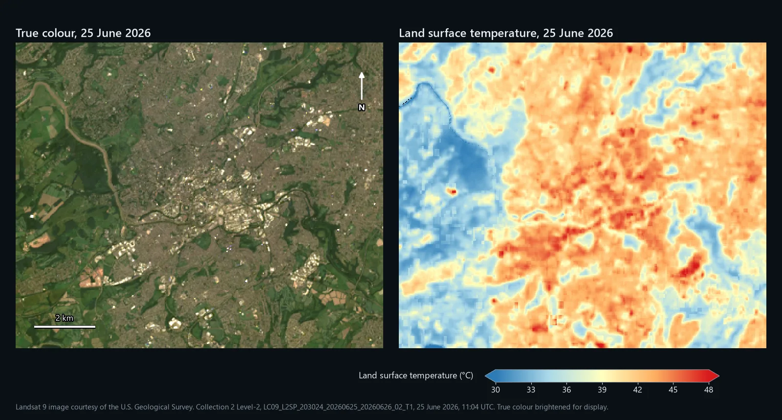
Map above: true colour and land surface temperature over a 12 by 10 km window of Bristol, from Landsat 9 at 11:04 UTC (12:04 BST) on 25 June 2026. Landsat 9 image courtesy of the U.S. Geological Survey. Collection 2 Level-2, LC09_L2SP_203024_20260625_20260626_02_T1, acquired 25 June 2026.
There are two ways to get land surface temperature (LST) into QGIS from Landsat 8 or 9. USGS already publishes it as a Level-2 product, and turning that into degrees Celsius takes one line in the Raster Calculator. Or you can work it out yourself from the thermal band with the single-channel method that many QGIS tutorials teach. This guide does both in QGIS 3.44, on one real scene, and shows how far apart they land and why.
The worked example is Bristol on 25 June 2026, a cloud-free Landsat 9 pass. Every map and number below comes from that scene. We scripted the figures in Python so they are reproducible, then ran the key steps again in QGIS 3.44.3 to check that the expressions printed here give the same answers.
What land surface temperature is, and is not
LST is the temperature of whatever the satellite sees from above: roofs, roads, the top of a tree canopy, grass, water. It is not air temperature, and on a sunny day the two can be far apart, because dark roofs and tarmac heat up much faster than the air above them. Across our window the median was 40.4 °C, and about one pixel in twenty was above 44.5 °C.
It is also a snapshot. Landsat 8 and 9 each pass over the UK at about 11:00 UTC, every 16 days apiece, so you get late morning on clear days only. The thermal band is measured at 100 m and delivered on the 30 m grid of the other bands, so a small park or a single roof will be blurred into its surroundings.
What you need
- QGIS 3.44. Any recent 3.x release works; menu names here are from 3.44.
- A free USGS account to download from EarthExplorer.
- Your area of interest as a polygon layer.
- A clear summer day. Cloud ruins thermal data even more than optical data, so be patient.
Step 1: find and download a Level-2 scene
- Sign in to EarthExplorer, set your area and a date range in Search Criteria, and keep the cloud cover low.
- Under Data Sets, tick Landsat > Landsat Collection 2 Level-2 > Landsat 8-9 OLI/TIRS C2 L2 and click Results.
- Check the browse image over your area, then use the download options to get the product bundle or just the files listed in step 2.
The product name tells you most of what matters. Ours was LC09_L2SP_203024_20260625_20260626_02_T1: Landsat 9 (LC09), Level-2 with surface temperature (L2SP), path 203 and row 24, acquired on 25 June 2026, processed on 26 June, Collection 2, Tier 1. The scene listed 4.25% cloud overall; over our window only 7 of 133,200 pixels were flagged.
Step 2: know which files you need
| File ending | What it holds | Used in |
|---|---|---|
_ST_B10.TIF | Surface temperature, scaled to whole numbers | Steps 4 to 7 |
_QA_PIXEL.TIF | Cloud, shadow and water flags | Step 5 |
_MTL.txt | Metadata, including every constant used below | Throughout |
_SR_B4.TIF | Surface reflectance, red | Step 10 |
_SR_B5.TIF | Surface reflectance, near-infrared | Step 10 |
_ST_TRAD.TIF | Band 10 converted to radiance at the sensor | Step 8 |
_ST_ATRAN, _ST_URAD, _ST_DRAD, _ST_EMIS | The atmosphere and emissivity USGS used | Step 12 |
Step 3: load and clip
Drag the files into QGIS and check the CRS in Layer Properties > Information. Landsat products come in WGS 84 / UTM; our path and row was zone 30 north, EPSG:32630. Then run Raster > Extraction > Clip Raster by Mask Layer on each file with your polygon as the Mask layer, tick Keep resolution of input raster, and use Run as Batch Process to do them all at once. In our files ST_B10 and the SR bands declared 0 as no data and the other ST_ bands -9999; Layer Properties > Information shows what yours declare.
Step 4: turn ST_B10 into degrees Celsius
ST_B10 stores temperature as whole numbers to keep the file small. Ours ran from 44,217 to 50,976. The _MTL.txt file gives the conversion to kelvin under TEMPERATURE_MULT_BAND_ST_B10 (0.00341802) and TEMPERATURE_ADD_BAND_ST_B10 (149.0). Open Raster > Raster Calculator and subtract 273.15 for Celsius:
Untick Create on-the-fly raster instead of writing layer to disk, save it as lst_c.tif and click OK. The output is 32-bit float, so the decimals survive. That is the whole of the USGS route: they have already corrected band 10 for the atmosphere and for the emissivity of the surface.
Step 5: mask cloud with QA_PIXEL
QA_PIXEL packs its flags into bits, and the Raster Calculator cannot test bits. It does not need to. For Landsat 8 and 9 Collection 2, a clear land pixel with low confidence of cloud, shadow, snow and cirrus has the value 21824, and the same over water 21952, so keep those two and drop everything else:
Each comparison returns 1 or 0, so the bracket is 1 for clear pixels and 0 for the rest, and QGIS returns NoData when dividing by zero. Save the result as lst_c_masked.tif. Run Raster analysis > Raster layer unique values report on QA_PIXEL first to see which values your window holds. Ours had three: 21824 (133,094 pixels), 21952 (99) and 22280 (7, all on the river near the north-west corner, flagged as cloud with high confidence). Decoding the bits properly in Python gave exactly the same mask.
Step 6: style it and read the values
- In Layer Properties > Symbology, set Render type to Singleband pseudocolor.
- Choose the RdYlBu ramp, tick Invert Color Ramp so that hot is red, and set Min to
30and Max to48.
Fixed values matter here for the same reason they do with NDVI: the default stretch fits each image to its own range, so two days styled that way cannot be compared by eye. The map at the top of this page uses exactly this ramp and range.
To see which surfaces run hot, we put ESA WorldCover 2021 land cover onto the same 30 m grid and took the median LST of each class. The first column of numbers is every pixel of that class; the second is only pixels sitting in a solid block of the class at least 210 m across, which takes the blur of the 100 m thermal band out of the picture.
| ESA WorldCover class | Median LST, all pixels | Median LST, solid blocks | Area in window |
|---|---|---|---|
| Built-up | 42.6 °C | 44.7 °C | 50.4 km² |
| Tree cover | 37.9 °C | 31.9 °C | 41.8 km² |
| Grassland | 36.0 °C | 34.7 °C | 25.0 km² |
| Water | 34.2 °C | too few pixels | 1.2 km² |
Tree cover reads warmer than grassland across all its pixels because, in a city, much of it is street trees and gardens mixed in with roofs. In solid blocks the order is what you would expect: woodland at 31.9 °C, grass at 34.7 °C and built-up ground at 44.7 °C, nearly 13 °C apart at the same moment.
Step 7: put a number on each area
A map shows the pattern; a report needs a number per area. For an even grid, open the Processing Toolbox and run Vector creation > Create grid with Grid type set to Hexagon (Polygon), the extent taken from lst_c_masked, and 500 for both Horizontal spacing and Vertical spacing, in the layer's CRS. Then run Raster analysis > Zonal statistics with the grid as the Input layer, lst_c_masked as the Raster layer, and Count and Mean ticked. Use your own boundaries instead, such as wards or LSOAs, if that is what your report needs.
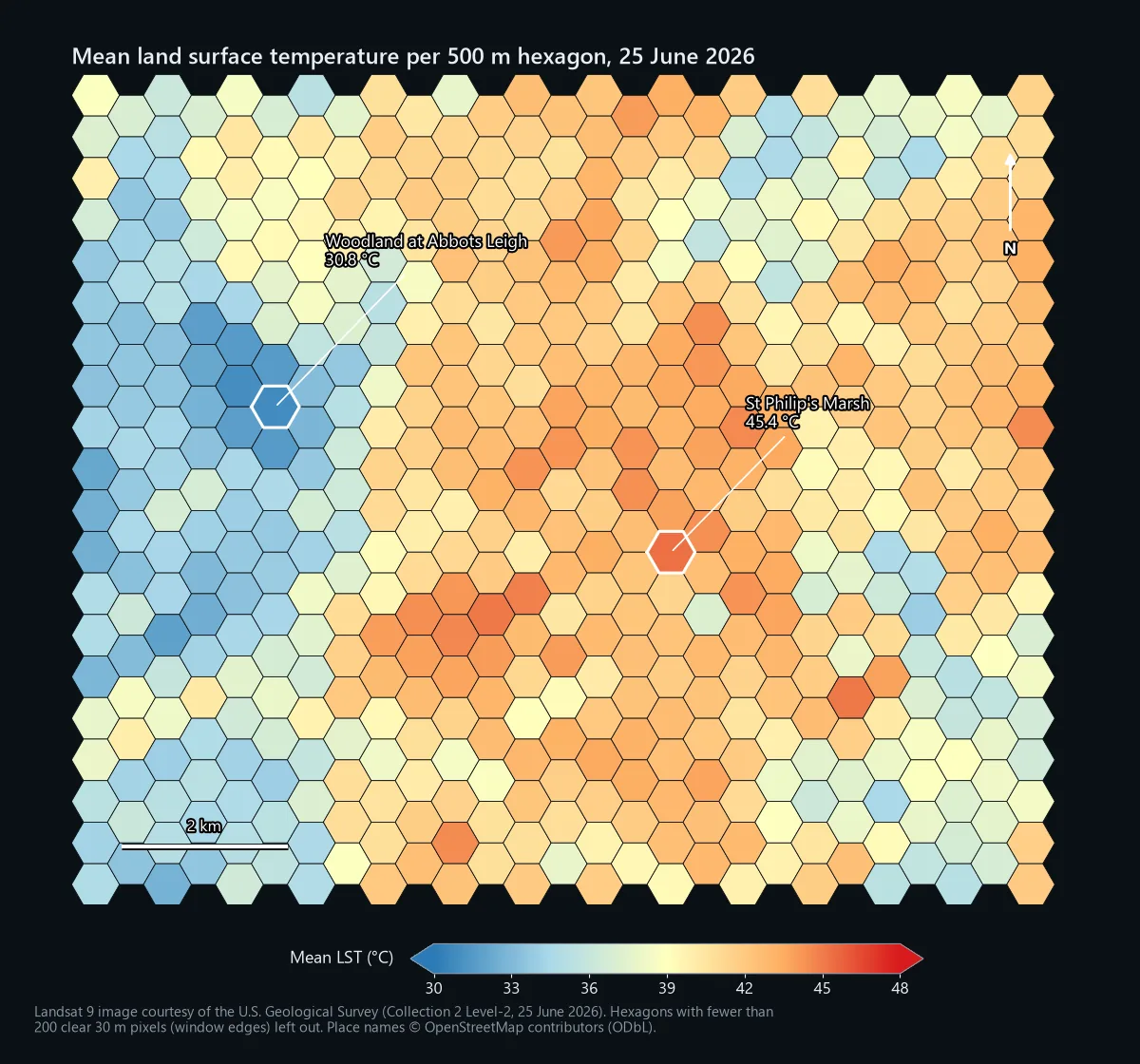
QGIS made 560 hexagons over our window, 527 of them with at least 200 clear pixels. Their means ran from 30.8 °C, over woodland at Abbots Leigh on the North Somerset side, to 45.4 °C over St Philip's Marsh, an area that ESA WorldCover classes as 99% built-up. The Count column tells you how many clear pixels went into each mean, so you can drop cells that are mostly cloud or edge.
Doing it by hand: the single-channel method
The Level-2 product is the better number, but plenty of people want or need to calculate LST themselves: for a course, for Level-1 data, or to understand what the product is doing. The single-channel method below is the one many QGIS tutorials use, and it is what our QGIS model automates.
Step 8: band 10 radiance
The Level-2 bundle already includes band 10 as radiance at the sensor, in watts per square metre per steradian per micrometre, scaled by 1,000:
Save it as radiance.tif. If you start from a Level-1 band 10 instead, the radiance is RADIANCE_MULT_BAND_10 * "B10@1" + RADIANCE_ADD_BAND_10, with both values from that product's MTL file. For our scene they were 0.00038 and 0.1.
Step 9: brightness temperature
Brightness temperature is what the satellite would read if the surface were a perfect emitter and there were no atmosphere. It uses two constants from the MTL, K1_CONSTANT_BAND_10 and K2_CONSTANT_BAND_10. For our Landsat 9 scene they were 799.0284 and 1329.2405:
The result is in kelvin; keep it that way and save it as bt_k.tif. Landsat 8 uses different constants (774.8853 and 1321.0789), so always copy them from your own MTL file.
Step 10: NDVI and emissivity
Real surfaces emit less than a perfect emitter, and vegetation emits differently from bare ground, so the method estimates emissivity from NDVI. The SR bands need their own scale and offset first (0.0000275 and -0.2, from REFLECTANCE_MULT_BAND_4 and REFLECTANCE_ADD_BAND_4, the same for band 5):
Save it as ndvi.tif and run Raster analysis > Raster layer statistics on it for the minimum and maximum. Ours were -0.098 and 0.899. The proportion of vegetation and the emissivity follow:
Save them as pv.tif and emissivity.tif. Using the window's own minimum and maximum is the common shortcut. Fixed thresholds of 0.2 for soil and 0.5 for full vegetation are the other common choice; on our scene the switch changed the final LST by 0.07 °C at the median, so it is not where the big differences come from.
Step 11: land surface temperature
Here 10.895 is the middle of band 10's 10.60 to 11.19 µm range, and 14388 is a physical constant (Planck's constant times the speed of light divided by Boltzmann's constant, in µm K). Brightness temperature must go in as kelvin. Save it as lst_hand_c.tif and mask it with QA_PIXEL as in step 5.
How it compared
Over our window the emissivity step added 0.86 °C at the median to the brightness temperature of 31.4 °C, giving a median LST of 32.2 °C. The USGS product said 40.4 °C. Pixel by pixel, the hand method came out 8.1 °C lower at the median, and between 5.2 and 9.7 °C lower for 90% of pixels. The pattern was the same, with a correlation of 0.991 between the two maps; the level was not.
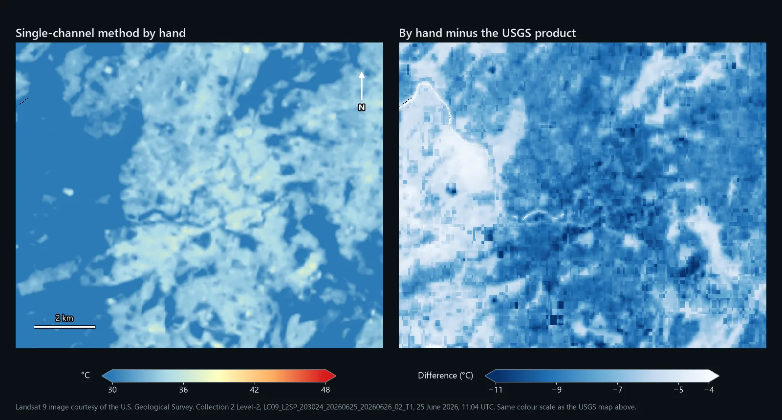
Step 12: where the 8 °C went
The single-channel method corrects for emissivity but not for the air between the ground and the satellite. Water vapour absorbs part of the thermal signal and the atmosphere adds some of its own. The Level-2 bundle includes the numbers USGS used for that correction, so you can close the gap yourself: transmittance (ST_ATRAN, scale 0.0001), upwelled and downwelled radiance (ST_URAD and ST_DRAD, scale 0.001) and emissivity (ST_EMIS, scale 0.0001). First the radiance leaving the surface:
Save it as surface_radiance.tif, then convert it with the same constants as step 9:
On our scene this came out 0.15 to 0.18 °C above ST_B10 for 90% of pixels. The median transmittance over the window was 0.62, so only 62% of the surface's band 10 signal reached the satellite directly. On a warm, humid June day that is a big effect, and it is the difference between the two methods. Use the hand method to understand LST or to compare places within one scene; use the Level-2 product when the temperature itself matters.
Common problems
Celsius in the emissivity step
Converting brightness temperature to Celsius before step 11 is an easy slip, and nothing errors. The emissivity correction just shrinks to almost nothing: on our scene it took 0.85 °C off the median LST. Keep kelvin until the very last subtraction.
Constants from the wrong satellite
Landsat 8 and Landsat 9 have different band 10 constants, and Level-1 radiance scaling can change between products. Copying them from a tutorial written for the other satellite gives a believable but wrong answer. Take them from your own MTL file every time.
Mixing up Level-1 and Level-2
ST_B10 is already temperature: putting it through the radiance and brightness temperature formulas gives nonsense. A Level-1 B10 is raw counts and needs steps 8 to 11. If your values are in the tens of thousands and your result is near absolute zero or far above 100 °C, check which product you loaded.
Comparing two dates
LST depends on the time of day, the sun, wind, recent rain and the season, so two dates are rarely directly comparable. Compare like with like (same month, similar weather), keep the fixed colour range from step 6, and consider mapping each pixel's difference from its own scene median as well as the raw values.
Expecting street-level detail
Band 10 is measured at 100 m. The 30 m pixels are a resampling, so a single roof, a narrow street or a small pocket park will not show its own temperature. For a building or a street you need airborne thermal data or a drone.
Credit the data
Landsat data from USGS is in the public domain. USGS asks for a credit line such as "Landsat 9 image courtesy of the U.S. Geological Survey", which we use on every map here. ESA WorldCover is licensed CC BY 4.0: credit "© ESA WorldCover project 2021 / Contains modified Copernicus Sentinel data (2021) processed by ESA WorldCover consortium". The place names on the hexagon map come from OpenStreetMap (© OpenStreetMap contributors, ODbL).
We ran it in QGIS 3.44.3 on this scene, with band 10 rebuilt from the radiance band because Level-1 files are a separate download. Left without atmospheric values, its median LST was 32.1 °C: 0.1 °C from our hand calculation and 8.2 °C below the USGS product, for the reason in step 12. It also takes three optional values for the atmosphere, one figure each for the whole scene: transmittance, upwelled radiance and downwelled radiance. With the medians of the Level-2 bundle's
ST_ATRAN, ST_URAD and ST_DRAD over our window (0.62, 3.20 and 1.47), its median came out at 39.6 °C, 0.6 °C below the USGS product, and between 2.1 °C below and 0.5 °C above it for 90% of pixels. Without those values, use it for patterns across an area; with them, it comes close to the USGS figure.It is a .model3 file with a PDF guide, for QGIS 3.34 or later, licensed CC BY-NC 4.0.