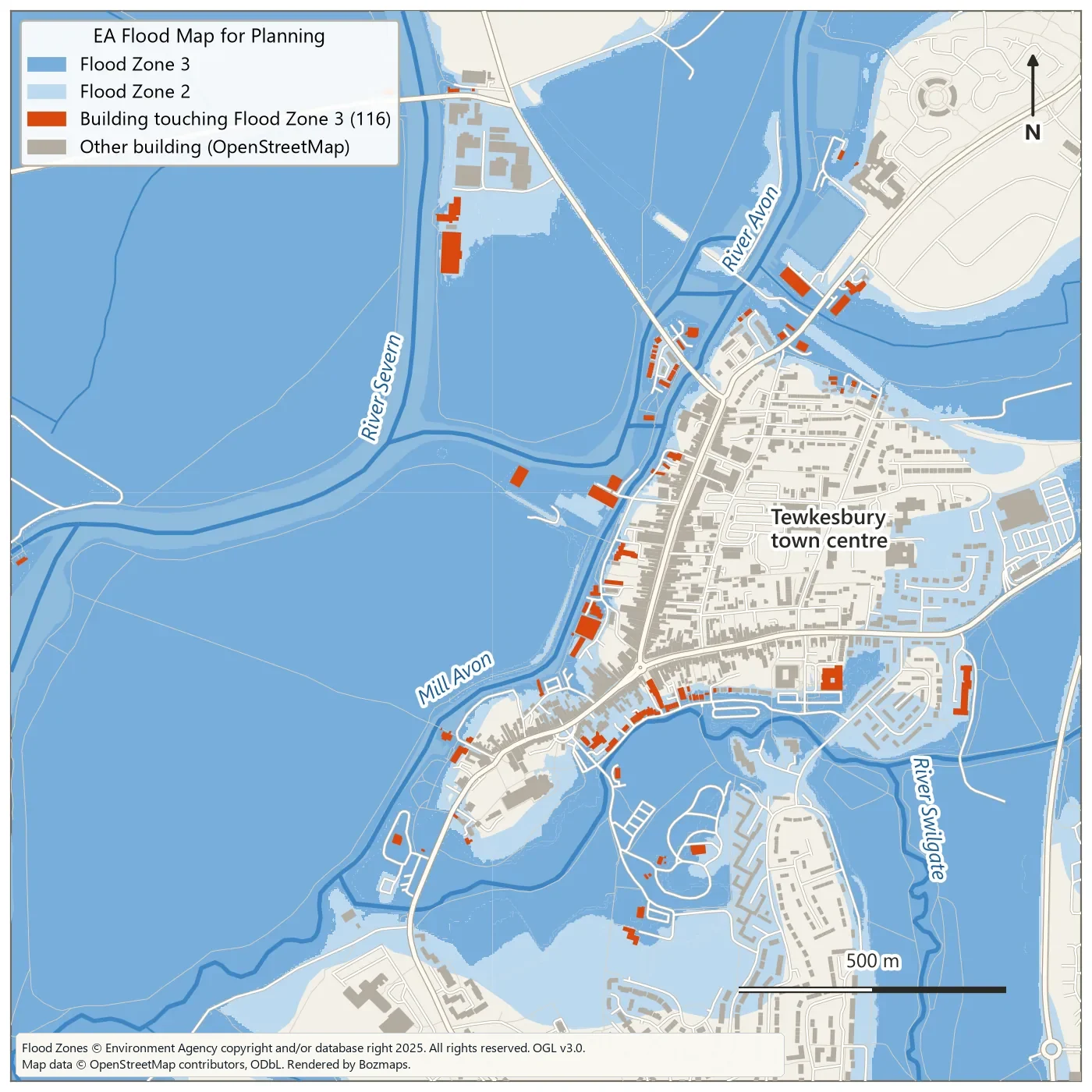
Map above: Environment Agency Flood Zones 2 and 3 across a 2 km square over Tewkesbury, with the 116 OpenStreetMap buildings that touch Flood Zone 3 in orange. Flood Zones © Environment Agency copyright and/or database right 2025. All rights reserved. Open Government Licence v3.0. Map data © OpenStreetMap contributors, ODbL.
Every river and stretch of coast in England already has official flood zones, so why build your own flood map in QGIS? The zones tell you how likely flooding is. A terrain model shows which ground lies below a given water level. Together they explain a place far better than either does alone.
This tutorial does both: overlay the Environment Agency (EA) flood zones on buildings, map land below a chosen water level from LiDAR, then wrap the terrain method in a Graphical Modeler model that reruns for any town and level. Every map and number below comes from running it on a 2 km square over Tewkesbury, where the Avon meets the Severn.
Two kinds of flood map
The EA's Flood Map for Planning puts land into flood zones. Flood Zone 3 has a 1% (1 in 100) or greater chance of flooding from rivers each year, or 0.5% (1 in 200) or greater from the sea. Flood Zone 2 sits between 0.1% and 1% for rivers (0.1% to 0.5% for the sea), and everything else is Flood Zone 1. The zones ignore the benefit of flood defences, and the EA states that the data is not suitable for showing whether an individual property is at risk.
The second kind is a terrain screening, often called a bathtub model: take a LiDAR elevation model, pick a water level and mark every cell at or below it. It knows nothing about rainfall, flow or defences, but it shows quickly and transparently which ground sits low relative to the river, at any level you choose, including a recorded flood level or one from EA modelling.
What you need
- QGIS 3.44, the current long term release. Every tool used here ships with QGIS. We used 3.44.3. The model in Step 7 needs 3.34 or later, because its Raster calculator step uses the Model Designer version of that tool, which arrived in 3.34.
- A study area polygon in British National Grid. Start with a few square kilometres.
- The EA LIDAR Composite DTM at 1 m for that area.
- Buildings and a river centreline, from Ordnance Survey or OpenStreetMap.
- The EA flood zones.
- Optional: the QuickOSM plugin, if you take buildings and rivers from OpenStreetMap.
Where to get the UK data
| Data | Where | Licence |
|---|---|---|
| Flood Zones 2 and 3 (England) | Flood Map for Planning, as downloads or an OGC API Features service | Open Government Licence v3.0 |
| Risk of flooding from rivers and sea, and from surface water | Rivers and sea and surface water on data.gov.uk | Open Government Licence |
| LIDAR Composite DTM, 1 m | Defra Survey Data Download, 5 km GeoTIFF tiles | Open Government Licence |
| Rivers and buildings | OS Open Rivers and OS OpenMap - Local from the OS Data Hub | Open Government Licence |
| Rivers, buildings, roads | OpenStreetMap, through QuickOSM | ODbL |
The flood zones were rebuilt on 25 March 2025 from the EA's new National Flood Risk Assessment and last updated on 22 October 2026. The LiDAR composite covers about 99% of England from surveys flown between 2000 and 2022, with heights in metres above Ordnance Datum Newlyn (m AOD from here on).
The EA data covers England only. Natural Resources Wales publishes a Flood Map for Planning on DataMapWales under the OGL, SEPA publishes flood maps for Scotland under OGL v3.0, and DfI Rivers runs Flood Maps (NI) for Northern Ireland.
Step 1: set the project to British National Grid
Open Project > Properties, go to the CRS tab and choose EPSG:27700 (OSGB36 / British National Grid). The EA and OS data are published in it, so distances and areas come out in metres. Load your study area polygon.
Step 2: load the flood zones
Open the Data Source Manager, choose the WFS / OGC API - Features tab and click New. Name the connection and paste the service's landing page as the URL:
Click OK, then Connect, select Flood Zones 2 3 Rivers And Sea, tick Only request features overlapping the view extent, zoom to your study area and click Add. Each feature has flood_zone (FZ2 or FZ3), flood_source and origin, which records whether the outline was modelled, recorded or both. Save the zones for your area to a GeoPackage in EPSG:27700 (right-click the layer, Export > Save Features As) so you are not hitting the server on every run.
Check the saved layer before you use it. In our test QGIS loaded the service in WGS 84, and after saving to EPSG:27700, 16 of the 73 outlines in our square had invalid geometry. QGIS Processing stops on invalid geometry by default, so run Fix geometries on the saved layer first. The trip through WGS 84 also shifts edges very slightly: we counted 115 buildings in Flood Zone 3 from those zones, against 116 from the EA GeoPackage, which is published in British National Grid.
Step 3: count the buildings in each zone
OS OpenMap - Local and OpenStreetMap both work for buildings. QuickOSM delivers WGS 84, so run Reproject layer to EPSG:27700 first.
In the Processing Toolbox, run Extract by attribute on the flood zones with Selection attribute flood_zone, Operator = and Value FZ3. Then run Extract by location with Extract features from set to your buildings, the predicate set to intersect, and By comparing to the features from set to the FZ3 layer. Repeat for Flood Zone 2.
In our Tewkesbury square, Flood Zone 3 covers 267 of the 400 hectares and 116 of the 1,546 OpenStreetMap buildings touch it. The Flood Zone 2 outlines do not overlap Flood Zone 3 and add another 52 hectares. Repeating the extraction for them returns 555 buildings, but 83 of those also touch Flood Zone 3, so Flood Zone 2 adds 472 buildings. OpenStreetMap outlines include garages and outbuildings, so read these as building counts, not homes.
Step 4: prepare the LiDAR
From the Defra Survey Data Download, select your area and download the LIDAR Composite DTM at 1 m. It arrives as one zip per 5 km Ordnance Survey grid square, each holding a GeoTIFF. Our square straddles two, SO83se and SO93sw. To join them, use Build virtual raster and untick Place each input file into a separate band, which is ticked by default.
Run Fill NoData on the DTM to patch small gaps, then Clip raster by mask layer with your study area as the mask, ticking Keep resolution of input raster. Fill first: Fill NoData interpolates into any empty cell within its search distance, including cells a clip has just blanked outside an irregular study area.
Step 5: find the river level
A recorded flood level, or modelled levels ordered from the EA, are the best sources. Without them, read the river surface from the LiDAR: Buffer your river line by 2 m, then run Zonal statistics on the buffer against the DTM with Minimum ticked under Statistics to calculate.
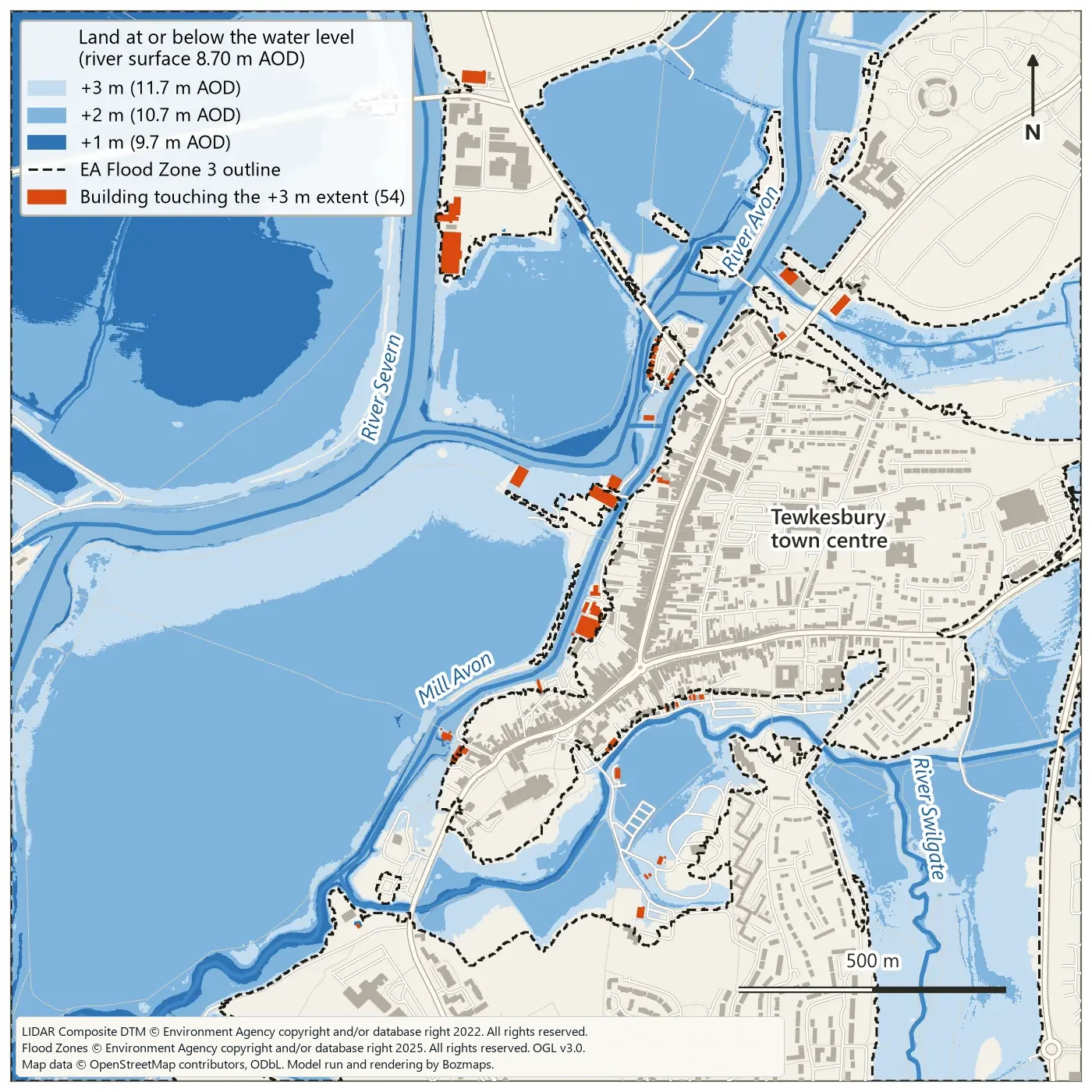
Topographic LiDAR does not see through water, so in the channel the DTM holds the water surface on the survey day, not the river bed. In Tewkesbury the lowest readings on the Severn and the lower Avon were both 8.70 m AOD, and one stretch of the Avon read 8.70 m end to end, which suggests the water was flattened when the composite was made. We used 8.70 m as the base and tested 1, 2 and 3 m above it. The ready-made model at the end of this article does this step for you.
Step 6: map the land below that level
Open Raster calculator from the Raster analysis group and enter an expression like this, using your own layer name:
Cells at or below 10.7 m become 1 and the rest 0. Run Polygonize (raster to vector), keeping the default field name DN, then Extract by attribute with DN = 1. That is your flood extent. Extract by location against the buildings, as in Step 3, gives the buildings it touches.
Step 7: build the model
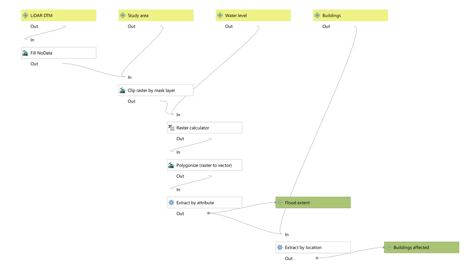
The Graphical Modeler chains those six tools into one tool with its own inputs. Open it from Processing > Model Designer and name the model under Model Properties.
Inputs
Drag these from the Inputs panel onto the canvas:
- Raster Layer called LiDAR DTM.
- Vector Layer called Study area, with Geometry type set to Polygon.
- Number called Water level, with Number type set to Float and a Default value of 10.
- Vector Layer called Buildings, with Geometry type set to Polygon.
Algorithms
Add these from the Algorithms panel. The dropdown beside each parameter sets its source: Value, Pre-calculated Value, Model Input or Algorithm Output.
| Algorithm | Settings |
|---|---|
| Fill NoData | Input layer: LiDAR DTM. Maximum distance: 100 pixels (the default is 10). |
| Clip raster by mask layer | Input layer: the Fill NoData output. Mask layer: Study area. Tick Keep resolution of input raster. |
| Raster calculator | Input layers: the clipped output. Expression: switch to Pre-calculated Value and enter concat('"A@1" <= ', @water_level) |
| Polygonize (raster to vector) | Input layer: the Raster calculator output. |
| Extract by attribute | Selection attribute DN, Operator =, Value 1. Set Extracted (attribute) to Model Output, named Flood extent. |
| Extract by location | Extract features from: Buildings. Predicate: intersect. Comparing to: the Extract by attribute output. Output named Buildings affected. |
Save and run
Save Model (Ctrl+S) writes a .model3 file. Saved in your profile's models folder, it appears in the Processing Toolbox under its group. To test several levels, right-click it in the Toolbox, choose Execute as Batch Process, and fill the Water level column with Autofill > Add Values by Expression using array(9.7, 10.7, 11.7), giving each row its own output names. The level is an absolute height in m AOD: enter 10.7, not 2.
What the Tewkesbury run produced
| Water level | Land at or below | Pieces | Touching a river | Buildings touched |
|---|---|---|---|---|
| +1 m (9.7 m AOD) | 59.7 ha | 371 | 24.4 ha in 15 pieces | 3 |
| +2 m (10.7 m AOD) | 187.1 ha | 1,079 | 124.8 ha in 1 piece | 11 |
| +3 m (11.7 m AOD) | 247.3 ha | 182 | 246.8 ha in 1 piece | 54 |
Three things stand out.
- The methods agree on where the low ground is. No land the model flagged falls outside Flood Zones 2 and 3 at any level, and at +3 m it covers 92% of Flood Zone 3.
- They disagree on buildings: 54 at +3 m against 116 in Flood Zone 3. The EA zones come from flood modelling and recorded outlines (Tewkesbury's
originfield shows both), so they reach ground that a flat 11.7 m level does not. - The +1 m result is mostly noise. 351 of its 371 pieces are under 100 m², and the largest, 33.7 ha of low ground in the north-west, touches no river line. Water would need a way in over a bank or through drains, and a bathtub model cannot tell you whether one exists.
A cheap partial fix is one more Extract by location that keeps only the pieces intersecting your river line. At +1 m that cut the extent from 59.7 ha to 24.4 ha.
Common problems
- CRS mismatches. QuickOSM and many web services give you WGS 84 (EPSG:4326). Buffer distances follow the layer's units, so a 2 m buffer on a layer in degrees becomes a 2 degree buffer. Reproject everything to EPSG:27700 first.
- Raster resolution. A 1 m DTM is a million cells per square kilometre: fine for a town, slow for a district, where the 2 m composite (also OGL) is a better start. Polygonize on 1 m cells makes thousands of slivers; Sieve (Raster analysis) removes small clumps first.
- Tiles in separate bands. Leave Place each input file into a separate band ticked in Build virtual raster and band 1 holds only your first tile.
- A slow flood zone service. While writing this, the EA's flood zone API sometimes took minutes or returned a 504 error, while small requests answered in under a second. If QGIS stalls, zoom in, or download the GeoPackage from the dataset page. That file covers all of England (about 1 GB zipped, 6.3 GB unzipped) and is in British National Grid.
- Buildings touched are not properties flooded. Extract by location counts any footprint that touches a flood polygon, whatever its floor level.
What this is not
This is a screening. A bathtub model ignores how water moves: no rainfall, flow paths, timing, defences or culverts, and one flat level that cannot follow a river falling downstream, so keep study areas short along the river. Use it to decide where to look harder, compare scenarios and explain risk. It is not a flood risk assessment.
In England, government guidance says you should complete a site-specific flood risk assessment for development in Flood Zones 2 and 3, for sites of 1 hectare or more in Flood Zone 1, and in several other cases, and that you will usually need to pay a flood risk specialist to do it. Specialists typically use the EA's detailed flood risk data, ordered through the Flood Map for Planning service, and often a 1D or 2D hydraulic model such as HEC-RAS that routes real flows over the terrain. For a single address in England, Check your long term flood risk covers rivers and the sea, surface water, reservoirs and, where data exists, groundwater.