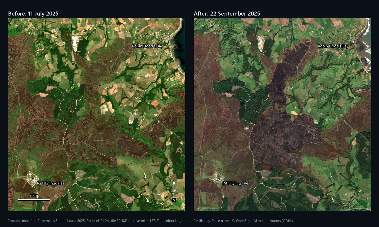
Map above: Fylingdales Moor on the North York Moors from Sentinel-2, on 11 July 2025 and on 22 September 2025, after the summer's fire. Contains modified Copernicus Sentinel data 2025. Place names © OpenStreetMap contributors (ODbL).
Mapping a burn scar in QGIS takes two satellite images, one band ratio on each and a subtraction. That is the differenced Normalised Burn Ratio, dNBR. Getting an area you can stand behind takes more: the right pair of dates, a threshold you have checked against the ground around the fire, and a comparison with someone else's figure. This guide covers all of it in QGIS 3.44 with free Sentinel-2 data.
The worked example is the 2025 fire on Fylingdales Moor, which the North Yorkshire Local Resilience Forum calls the largest wildfire in the recorded history of the North York Moors National Park. According to the forum's report on the response, it was first reported in Langdale Forest on 26 June, flared up again on 11 August, and on 25 August broke through a firebreak and ran north across the moor. The fire service kept major incident status until 23 September. Every number and map below comes from Sentinel-2 images either side of it, put through the steps in this guide.
What NBR and dNBR measure
Healthy vegetation reflects a lot of near-infrared (NIR) light. Burnt ground reflects much less NIR and more shortwave infrared (SWIR), the longer wavelengths that respond to water content and charcoal. The Normalised Burn Ratio turns that into one number per pixel:
Both are set out in Key and Benson (2006), the FIREMON Landscape Assessment chapter written for the US Forest Service. Burnt ground drops in NBR, so a high positive dNBR means a big change. On Sentinel-2, use band 8A (narrow NIR) and band 12 (SWIR2), both at 20 m. Inside our fire, the median NBR fell from 0.42 before to -0.33 after, a median dNBR of 0.74.
What you need
- QGIS 3.44. Every tool here ships with QGIS.
- A free Copernicus Data Space Ecosystem account for Copernicus Browser. Our NDVI guide walks through the download.
- The fire's dates from fire service or news reports, so you can choose images either side of it.
- A study window a few kilometres bigger than the fire on every side. You need unburnt ground around it for step 6.
Step 1: choose the two dates
The image after the fire should come once it is out or contained, on a clear day, before vegetation starts to grow back. The image before should be clear, from before the fire started, and ideally at a similar time of year so that the vegetation is at the same stage. Both should share a tile and, if possible, a relative orbit, so the pixel grids match and the viewing angle is the same.
Our pair, both tile T30UXF and relative orbit 137:
| Role | Date | Product |
|---|---|---|
| Before | 11 July 2025 | S2A_MSIL2A_20250711T110651_N0511_R137_T30UXF_20250711T153113 |
| After | 22 September 2025 | S2B_MSIL2A_20250922T110659_N0511_R137_T30UXF_20250923T075628 |
The fire had been contained since 27 August, according to a fire service update on 18 September. When it was first reported in June it measured about 100 m by 100 m; anything burnt before 11 July already looks burnt in the before image, so dNBR will not count it. Later we test a pre-fire image from a year earlier, which is the textbook choice, and show why it did worse here.
Step 2: load and clip the bands
From each product, take B8A, B12 and SCL from GRANULE/.../IMG_DATA/R20m. All three are 20 m, so nothing needs resampling. Check the CRS in Layer Properties > Information: tile 30UXF is WGS 84 / UTM zone 30N, EPSG:32630. Then run Raster > Extraction > Clip Raster by Extent (or by mask layer) on each band, with 0 as the NoData value. Our window was 11 by 12 km, 550 by 600 pixels. Name them B8A_jul, B12_jul, B8A_sep, B12_sep and so on.
Step 3: check for the reflectance offset
Since processing baseline 04.00 (January 2022), ESA adds 1,000 to every L2A reflectance value. Both our products are baseline 05.11 (N0511), so the raw files from Copernicus Browser carry it. It matters for NBR exactly as it does for NDVI: the difference on top is unchanged, but the sum underneath is 2,000 too big, which pulls every value towards zero.
Check with Identify Features on open water in B8A: around 1,000 means the offset is in, close to zero means it has been removed. The NDVI guide has the full check. We read our bands from the Earth Search catalogue on AWS, whose copies already have it removed: open water in our July B8A had a median value of 1.
Step 4: calculate NBR for each date, then dNBR
Open Raster > Raster Calculator. If the offset has already gone:
If step 3 says the offset is in:
Untick Create on-the-fly raster instead of writing layer to disk, save it as nbr_jul.tif, and do the same for September as nbr_sep.tif. Then subtract, before minus after, so that burnt ground comes out positive:
Save it as dnbr.tif. Key and Benson treat values below about -0.55 or above 1.35 as anomalies rather than fire effects. We had 3,552 such pixels, 3,281 of them on the sea in the north-east corner.
Step 5: classify burn severity
Key and Benson give seven example severity levels, published on a scale multiplied by 1,000; divided by 1,000 they become the rows below. Run Raster analysis > Reclassify by table on dnbr with these rows, and set Range boundaries to min <= value < max:
| Minimum | Maximum | Value | Severity level | Inside our fire |
|---|---|---|---|---|
| -10 | -0.25 | 1 | Enhanced regrowth, high | 2.1 ha |
| -0.25 | -0.10 | 2 | Enhanced regrowth, low | 11.2 ha |
| -0.10 | 0.10 | 3 | Unburned | 23.9 ha |
| 0.10 | 0.27 | 4 | Low severity | 50.2 ha |
| 0.27 | 0.44 | 5 | Moderate-low severity | 154.1 ha |
| 0.44 | 0.66 | 6 | Moderate-high severity | 394.8 ha |
| 0.66 | 10 | 7 | High severity | 1,069.0 ha |
The -10 and 10 just close the open-ended rows. The last column is our result inside the outer edge of the fire polygon from step 6, 1,705 ha in all; the unburned and regrowth hectares are islands inside it.
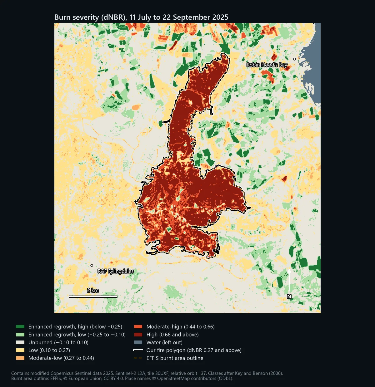
Treat the classes as a guide. Key and Benson write that the ranges are flexible and depend on the image pair, that thresholds can shift by about 0.1, and that they should be calibrated against field plots (their Composite Burn Index). They built the scale in the forests and shrublands of the western United States. On a peat moor, dNBR tells you how much the surface changed, not how deep the peat burned.
Step 6: draw the fire boundary and measure it
Low severity starts at 0.10, but that is not a safe line for drawing a fire boundary. First look at how much the ground away from the fire changed. Across every clear pixel more than 500 m outside our fire, the median dNBR was 0.02, but 26.3% of those pixels were 0.10 or above; the severity map shows fields and moor changing between July and September too. Only 2.7% were 0.27 or above, so we drew the boundary at 0.27.
- Raster Calculator:
"dnbr@1" >= 0.27, saved asburned.tif. Burnt pixels become 1, the rest 0. - Raster analysis > Sieve with Threshold 25, which removes clumps smaller than 25 pixels (1 ha at 20 m). Leave Use 8-connectedness unticked.
- Raster conversion > Polygonize (raster to vector) on the sieved layer, keeping the field name
DN. - Add a point on the burn scar to a new layer, then run Vector selection > Extract by location to keep the polygon that intersects it.
- Vector geometry > Add geometry attributes with Calculate using set to Layer CRS gives the area in square metres. Divide by 10,000 for hectares.
We ran these steps in QGIS 3.44.3 and got one polygon of 1,649.4 ha, with 26 holes for unburnt islands. The threshold matters: at 0.10 the polygon spread into the moor and fields around the fire and measured 3,590 ha; at 0.44 it shrank to 1,500 ha.
Step 7: check it against someone else's figure
Two independent sources map this fire. The European Forest Fire Information System (EFFIS) publishes burnt area outlines for fires across Europe, including the UK, and you can load them in QGIS as a WFS layer from https://maps.effis.emergency.copernicus.eu/effis (layer ms:modis.ba.poly). Its outline for this fire measures 1,677 ha. Our polygon covers 94.9% of it, and 96.5% of our polygon lies inside it; on the severity map above the two lines almost sit on top of each other.
The Local Resilience Forum's report gives 1,467 ha as the burn area on Fylingdales Moor and an estimated 200 ha of Forestry England land affected, and says the fire boundary covered about 20 square kilometres at its peak. Those figures come from different methods and dates, so they will never match to the hectare, but ours sits squarely among them. If your polygon came out at twice everyone else's, you would know to look again at the threshold or the dates.
Choosing the pre-fire date: a test
Key and Benson recommend matching the season of the two images, so that unburnt vegetation looks the same in both. The textbook move would have been a pre-fire image from September 2024, a year before the after image. We tried it with 17 September 2024 (Sentinel-2B, same tile and orbit), ran exactly the same steps, and got 1,941 ha, 292 ha more.
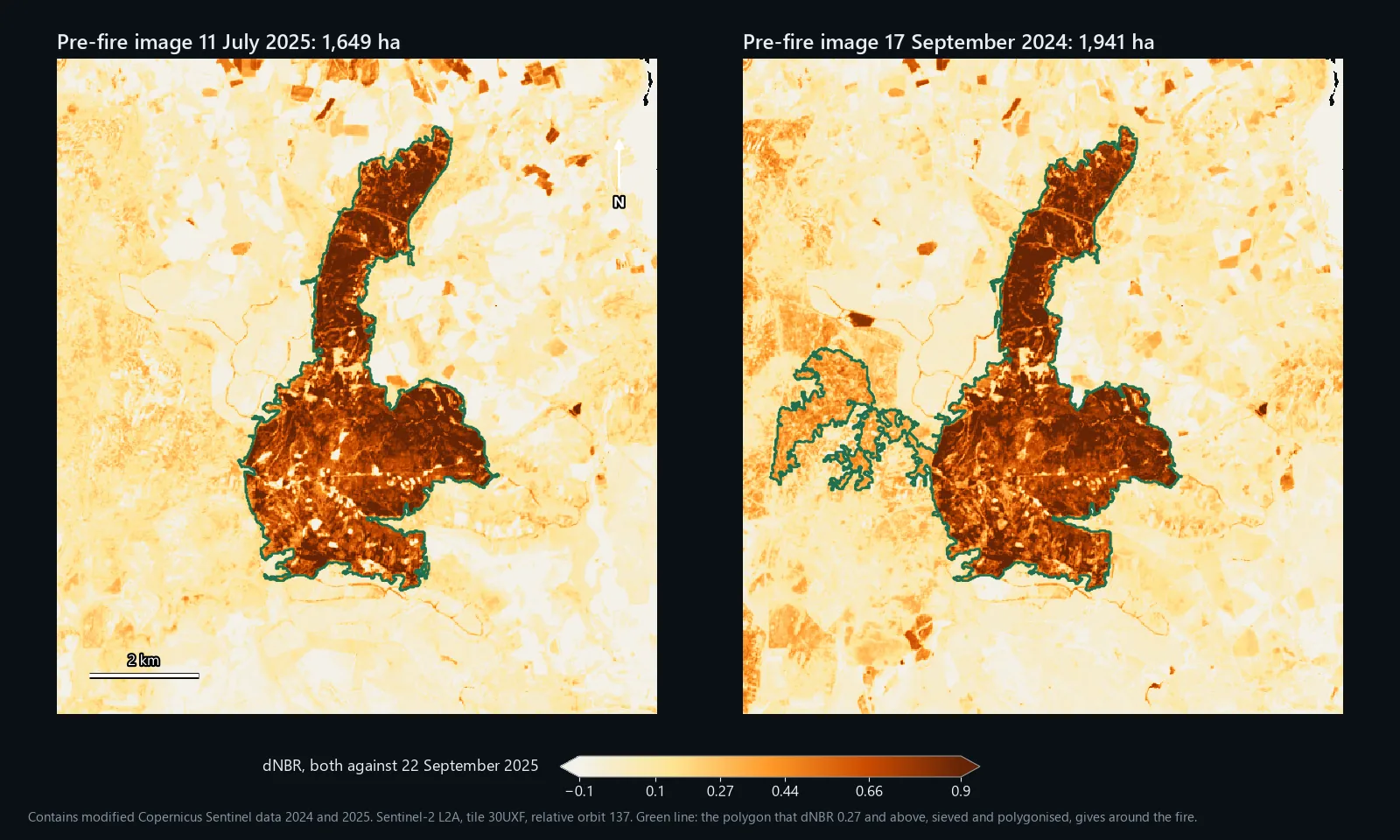
Most of the difference, 270 ha, is a block of moor west of the fire, outside the EFFIS outline and with no burn scar in the imagery. Its NBR fell steadily through 2025, from 0.46 in September 2024 to 0.25 in July 2025 and 0.08 in September 2025, so against the year-earlier image it scored a median dNBR of 0.36 without burning. Away from the fire, the share of pixels at 0.27 or above rose from 2.7% to 8.0%. Key and Benson warn about this: when the after image is drier than the before image, unburnt vegetation starts to look like a light burn. Their other condition matters too: the before image must not span other disturbances, and a year is plenty of time for those.
Neither choice is always right. Same season is the better default; a recent image is better when the landscape changed during the year. Run both if you can, and if they disagree, look at the imagery to see why.
Common problems
Forgetting the offset
Nothing errors; the burn just looks milder. We added the 1,000 back to our bands, as they sit in the raw files, and ran the plain formula. The median dNBR inside the fire fell from 0.74 to 0.41, and the area classed as high severity from 1,069 ha to 27 ha. Step 3 catches it.
Masking burnt ground by mistake
The SCL band is useful for cloud, but it was not built for burn scars. On 22 September it called 90.5% of the burnt ground "not vegetated", which is fair, and 5.3 ha of it "water". It called none of it cloud shadow this time, but dark burnt ground can look like shadow, so check before you mask. We dropped only SCL classes 0, 1, 3, 8, 9 and 10 (no data, defective, cloud shadow, cloud and cirrus) on either date, which removed 0.03% of the window and nothing inside the fire.
Farmland that looks like fire
A field harvested between the two dates loses NIR and gains SWIR just like burnt heather. That is why step 6 keeps only the polygon you clicked on rather than every pixel above the threshold, and why the map outside the fire should not be read as severity.
Band 8 instead of band 8A
Band 8 is 10 m and wider; band 8A is 20 m, narrower and the same size as band 12. Some workflows, including our model below, use band 8. On this fire it made almost no difference: with band 8 averaged to 20 m, the polygon came out at 1,654 ha against 1,649 ha. If you use band 8, set the Raster Calculator's output to 20 m pixels so the two bands share one grid.
One image instead of two
NBR below zero on the after image alone is a quick way to spot a fresh burn. On our 22 September image it picked up 88.6% of the fire polygon, but also 304 ha outside it in 842 separate patches, 97% of which the SCL called "not vegetated". It gives you no severity and no way to separate the burn from bare fields, tracks or quarries without the before image.
Credit the data
Copernicus Sentinel data is free, full and open; for maps like these use "Contains modified Copernicus Sentinel data [Year]". EFFIS content is © European Union and licensed CC BY 4.0, so credit EFFIS and say if you changed it. Place names on our maps come from OpenStreetMap (© OpenStreetMap contributors, ODbL). The fire's history and the official areas come from the North Yorkshire Local Resilience Forum's report, linked above.
Two differences from this guide. It uses band 8 rather than band 8A, which made almost no difference on this fire (see above). And it keeps every patch above the threshold inside your study area, not just the one you click, so draw the study area tightly around the fire. In the model's own test on the 2018 Saddleworth Moor fire, a study area around the moor gave 1,103 ha burned; a 12 by 12 km box that also took in fields around Mossley and Stalybridge gave 2,171 ha, most of the extra from fields and bare ground. It uses the bands as supplied, so remove the offset first if step 3 says so.
It is a .model3 file with a PDF guide, for QGIS 3.34 or later, and needs the QuickOSM plugin and an internet connection. Licensed CC BY-NC 4.0.