A landslide susceptibility map answers one question: given the ground, where are slopes most likely to fail? This tutorial builds one in QGIS with a weighted overlay of seven factors, then does the part most tutorials skip, which is testing the result against landslides that have actually happened.
We ran every step below over a 14.6 km by 12.2 km window of the Peak District around Edale, Mam Tor and the Hope Valley, where the British Geological Survey holds 185 landslide records. The window runs from 406740, 379290 to 421350, 391440 on the British National Grid (EPSG:27700). The processing ran in QGIS 3.44 on free data only, with Copernicus GLO-30 for elevation so the same steps work outside England, and every number and figure below comes from that run.
Susceptibility is not hazard, and it is not risk
Susceptibility ranks places by how likely a landslide is, given terrain, geology and other conditions. Hazard adds how often and how big. Risk adds what is in the way and how badly it would be damaged. Fell et al. (2008) set out these definitions for land-use planning, and they are worth reading before anyone writes "risk" on a map.
A weighted overlay is a desk screening tool. It tells you where to look harder. It never replaces a site walkover or a ground investigation by a qualified engineering geologist.
What you need
- QGIS 3.44. Everything here uses tools that ship with it. The curvature step uses the GRASS provider, which comes as the core "GRASS GIS Processing Provider" plugin; if the GRASS group is missing from the Processing Toolbox, enable it under Plugins. No SAGA tools are needed.
- An area of interest polygon in a projected coordinate system measured in metres.
- The data below. All of it is free; the licences differ, so note them as you go.
| Layer | Source | Licence |
|---|---|---|
| Elevation (England) | EA LIDAR Composite DTM, 1 m, about 99% of England | Open Government Licence |
| Elevation (anywhere) | Copernicus DEM GLO-30 | Free licence, fixed attribution text |
| Geology | BGS Geology 625k | Open Government Licence |
| Land cover | ESA WorldCover 2021, 10 m | CC BY 4.0 |
| Rivers and roads | OS Open Rivers (GB) or OpenStreetMap | OGL v3 / ODbL |
| Rainfall (large areas) | HadUK-Grid, 1 km | Open Government Licence |
| Landslide inventory | BGS National Landslide Database (index) | OGL for the index; full database licensed |
Three cautions. Copernicus DEM is a surface model, so woodland edges and buildings show up as steep ground; in England, use the LiDAR terrain model if you can. BGS Geology 50k beats 625k at valley scale, but the full dataset is licensed for commercial use (you can view it free). And BGS GeoSure landslides is a licensed susceptibility product in its own right, separate from the free inventory.
Step 1: put everything on one grid
Every factor must share the same coordinate system, cell size and extent, so that each cell in the final sum refers to the same patch of ground. Pick a projected CRS in metres (EPSG:27700 in Great Britain, a UTM zone elsewhere) and a cell size that suits your coarsest important layer.
Open GDAL > Raster projections > Warp (reproject) in the Processing Toolbox. Set the target CRS and an output resolution of 30, then open Advanced Parameters and give every layer the same Georeferenced extents of output file to be created. Use Bilinear resampling for the DEM and Mode or Nearest Neighbour for categories such as land cover. Our grid came out at 487 by 405 cells. Raster tools > Align rasters will snap several layers to a reference in one go.
Step 2: derive slope, aspect and curvature
Run Raster terrain analysis > Slope and Aspect on the projected DEM. Both output degrees, with aspect measured clockwise from north, 0 to 360.
For curvature, run GRASS > Raster (r.*) > r.slope.aspect and save the Tangential curvature output. GRASS writes curvature in 1/metres, with convex ground positive and concave ground negative. Tangential curvature measures how flow converges across a slope, and hollows that gather water are a common starting point for shallow slides. Profile curvature is a reasonable alternative.
Step 3: geology, land cover and distance layers
Geology. Give each polygon a score with the Field calculator, then burn it into a raster. In this part of the Peak District, the large slides such as Mam Tor happen where sandstone sits on weak mudstone of the Edale Shales, which the 1:625,000 map groups into the Bowland High Group and Craven Group. So that unit scores highest:
The ELSE 1 line catches every unit you have not named, so check the list of LEX_D values for your own window first. Less than 4 km east or west of ours, the same expression would score the Pennine Lower Coal Measures, which are rich in mudstone, as 1.
Then run GDAL > Vector conversion > Rasterize (vector to raster) with that field as the burn-in value, output size units set to Georeferenced units, width and height 30, and the DEM's extent.
Land cover. Warp ESA WorldCover onto your grid with Mode resampling. Its class codes are fixed: 10 tree cover, 20 shrubland, 30 grassland, 40 cropland, 50 built-up, 60 bare or sparse vegetation, 80 water, 90 wetland, 100 moss and lichen, and so on. Run Raster analysis > Raster layer unique values report on the warped layer to see which codes your window holds (ours had 10, 30, 40, 50, 60, 80 and 90), because every one of them needs a row in the reclassification table.
Distance to rivers and roads. Rasterize each line layer with a fixed burn value of 1 and the advanced "Pre-initialize the output image with value" set to 0. Then run GDAL > Raster analysis > Proximity (raster distance) with 1 as the target pixel value and Distance units set to Georeferenced coordinates. We used OpenStreetMap ways tagged waterway=river or waterway=stream (430 km inside the window) and public roads from motorway down to unclassified and residential, with their link roads (147 km, leaving out farm tracks, service roads and paths).
Rainfall earns its place when it varies meaningfully across the study area. Over one valley it adds little, so we left it out; for a county or a country, add HadUK-Grid like any other continuous factor.
Step 4: reclassify every factor to the same 1 to 5 scale
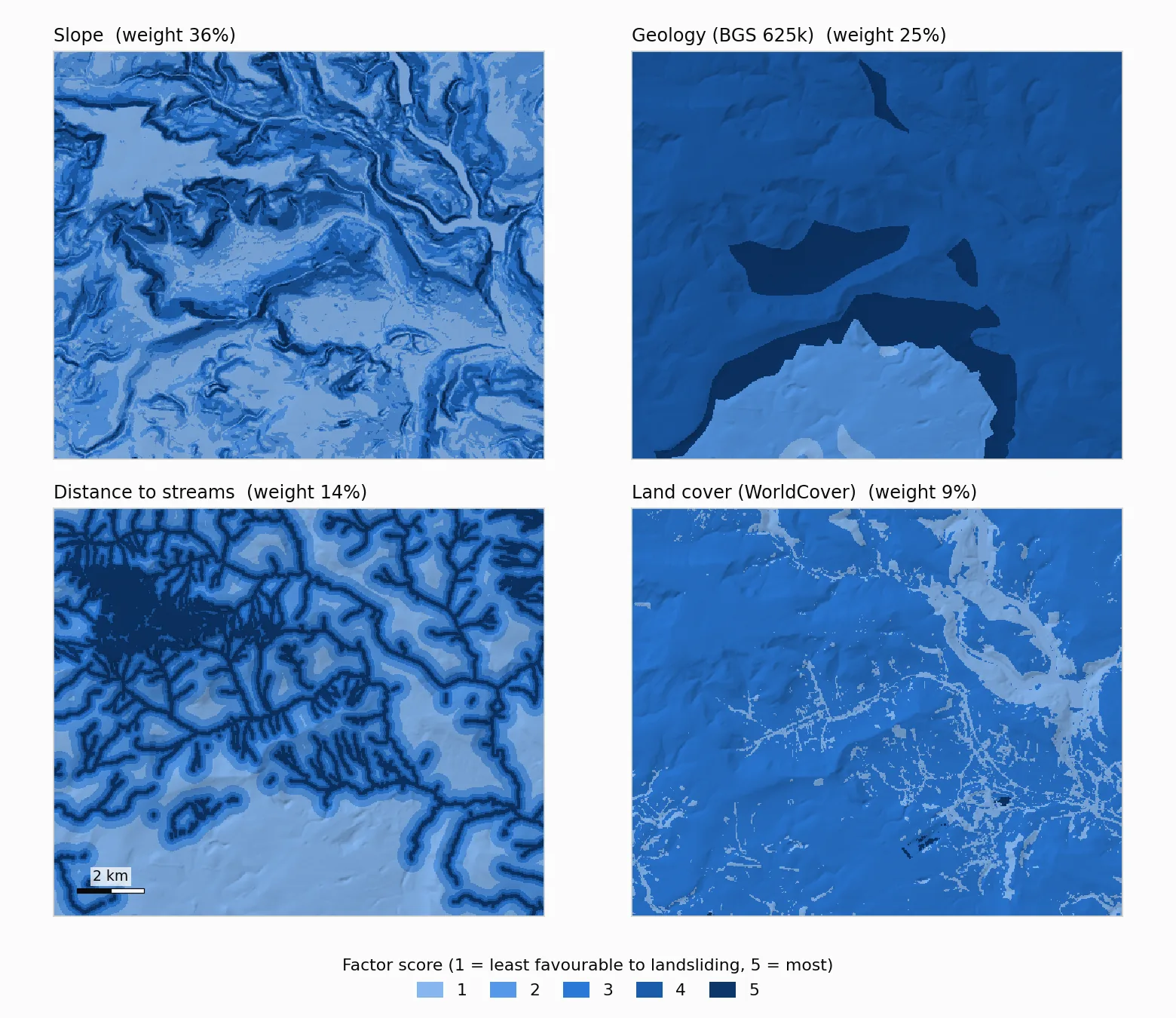
Slope in degrees, distance in metres and geology codes cannot be added together. Reclassifying puts them on one scale, where 1 is least favourable to landsliding and 5 is most. These are the breaks we used. They are judgement calls for this terrain, and yours should come from the literature for your area.
| Factor | Scores (1 = low, 5 = high) |
|---|---|
| Slope (degrees) | under 5 = 1, 5 to 10 = 2, 10 to 15 = 3, 15 to 25 = 4, 25 and over = 5 |
| Geology | igneous rocks 1, limestone 2, Millstone Grit 4, Bowland and Craven mudstones 5 |
| Distance to streams (m) | under 50 = 5, 50 to 100 = 4, 100 to 200 = 3, 200 to 400 = 2, 400 and over = 1 |
| Land cover | trees and water 1, shrubland 2, grassland, cropland, built-up and wetland 3, bare ground 5 |
| Tangential curvature (1/m) | concave (below -0.001) 5, planar 3, convex (above 0.001) 1 |
| Distance to roads (m) | under 50 = 5, 50 to 100 = 4, 100 to 250 = 3, 250 to 500 = 2, 500 and over = 1 |
| Aspect (degrees) | north-facing (315 to 360 and 0 to 45) 3, east (45 to 135) and west (225 to 315) 2, south (135 to 225) 1 |
Use Raster analysis > Reclassify by table. Enter one row per range (minimum, maximum, value), then open the advanced parameters and make two changes. Set Range boundaries to min <= value < max so zero and every class edge are caught once. And tick Use NoData when no range matches value, for reasons covered under common problems.
Two score layers will have gaps. Aspect leaves flat ground as NoData, and r.slope.aspect leaves the outer ring of cells empty. Run Raster tools > Fill NoData cells on the aspect and curvature scores with a Fill value of 3, the middle of the scale, or every gap becomes a hole in the final map.
Step 5: weight the factors with AHP
The Analytic Hierarchy Process turns weighting into a series of small decisions. Saaty (1990) describes the method: compare each pair of factors on a 1 to 9 scale (1 equal importance, 3 moderate, 5 strong, 7 very strong, 9 extreme), take the principal eigenvector of that matrix as the weights, and check the consistency ratio (CR). Saaty treats a CR under 0.10 as consistent enough to use; above that, some of your judgements contradict each other and need another look. Seven factors need 21 comparisons, and a few lines of Python in the QGIS Python Console do the maths:
Our judgements give slope 0.36, geology 0.25, distance to streams 0.14, land cover 0.09, curvature 0.08, distance to roads 0.05 and aspect 0.03, with a CR of 0.014. We set these before looking at the inventory, which matters in Step 7.
Step 6: combine and classify
Open Raster analysis > Raster calculator, add the seven score layers and enter the weighted sum:
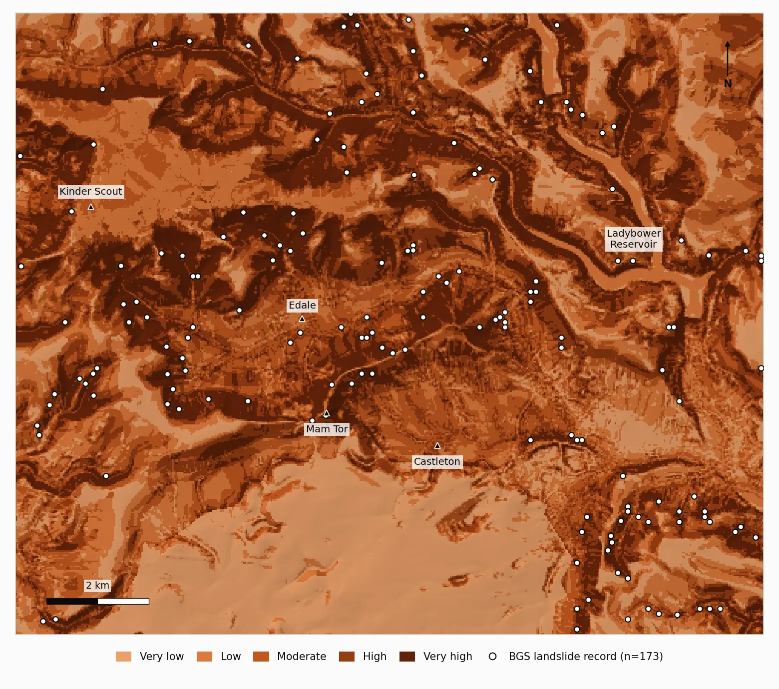
Because the weights sum to 1, the result stays on the 1 to 5 scale; ours ran from 1.15 to 4.51. To split it into classes, open the layer's Symbology, choose Singleband pseudocolor, set Interpolation to Discrete, the mode to Quantile and the classes to 5, click Classify and read off the first four values (ours were 2.41, 2.71, 3.01 and 3.36). Leave Interpolation on its default of Linear and QGIS lists the minimum, the quartiles and the maximum instead (1.15, 2.52, 2.85, 3.26 and 4.51 here). Feed the four breaks into Reclassify by table to produce a class raster from 1 (very low) to 5 (very high). Quantile classes each cover about a fifth of the area (19% to 22% here, because many cells share the same score), which makes the validation easy to read. Equal interval or natural breaks are also common; whichever you use, say so on the map.
Step 7: check it against a landslide inventory
A susceptibility map that has never been compared with real landslides is an opinion with a colour ramp. The check is simple: landslide locations should score higher than random locations.
- 1. Get and filter the inventory. BGS serves the free index as an OGC API Features collection at
https://ogcapi.bgs.ac.uk/collections/landslideindex; add it withLayer > Add Layer > Add WFS / OGC API - Features Layeror download GeoJSON for your box from its items link. The index places each record at the highest point of the backscarp where it can, but some older records are only located to the nearest kilometre. We kept records checked by BGS and located to 100 m or better withExtract by expressionand"grid_checked_by_bgs" = 'Y' AND "plus_or_minus_metres" <= 100, which left 173 of the 185 in the window. - 2. Make background points.
Bufferthe records by 250 m with Dissolve result ticked, useDifferenceto remove that from your study area, then runRandom points in polygonsfor 1,000 points. Set the Random seed under Advanced Parameters (we used 42) so you can repeat it. - 3. Sample the map. Run
Sample raster valueson both point layers against the continuous susceptibility raster. Each gets aSAMPLE_1column. Export both as CSV. - 4. Calculate the AUC.
The AUC is the area under the ROC curve, which plots the share of landslides you would catch against the share of background you would wrongly flag, at every possible cut-off. An AUC of 0.5 is no better than chance and 1.0 is perfect. It also has a plain reading: the probability that a randomly chosen landslide location scores higher than a randomly chosen background location. Reichenbach et al. (2018) review how susceptibility models are built and checked, and are a good next read.
For the class view, count records per class with Sample raster values on the class raster, and get area per class from Raster layer unique values report.
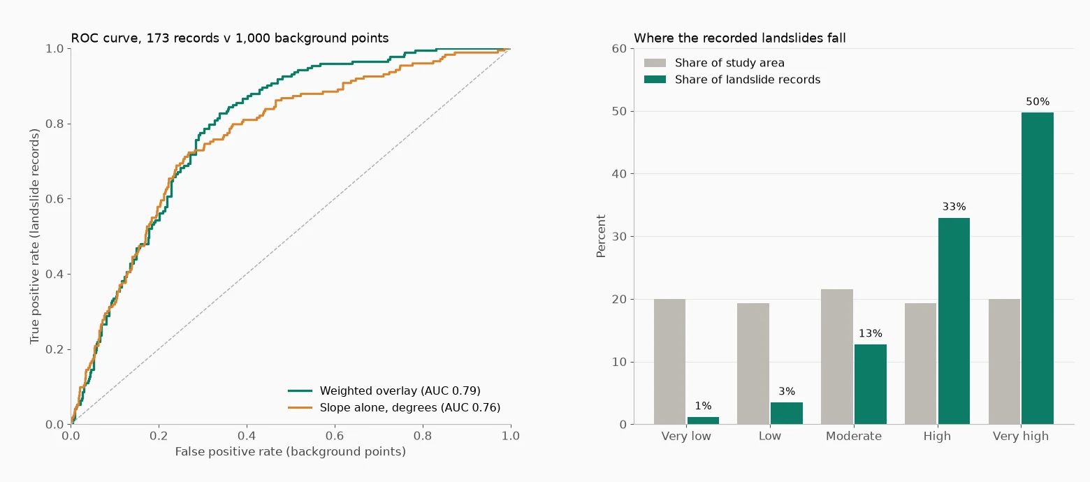
What our run showed. The AUC was 0.79 across all 173 records and 0.84 for the 75 records located to within 10 m, which suggests location error drags the headline figure down. The very high class covers 20% of the window and holds 86 records (50%). High and very high together cover 39% of the area and hold 143 records (83%), while the two lowest classes cover 39% and hold 8 records (5%).
The background sample moves these numbers a little. Repeated with ten different seeds, the AUC ranged from 0.79 to 0.81 for all records and from 0.84 to 0.86 for the 10 m records, so treat the second decimal place as approximate and quote the seed with your result.
The less flattering finding is just as useful. Raw slope on its own scores 0.76, so the other six factors add about 0.03 (between 0.025 and 0.033 across the ten seeds). Tested one at a time, geology (0.57 to 0.60 across the seeds) and distance to streams (0.57 to 0.60) carry some signal. Curvature (0.52 to 0.54), distance to roads (0.47 to 0.50) and aspect (0.49 to 0.52) sit close to chance, and land cover (0.44 to 0.46) falls just below it, so its scores slightly favour ground with fewer recorded slides. The 1:625,000 geology is the first thing we would upgrade.
The trap is to now re-weight the factors until the AUC rises. Do that on the same records and you are marking your own homework. Hold back part of the inventory, by a random split or by area, and test only on records the weighting never saw. Chung and Fabbri (2003) set out this distinction between success-rate and prediction-rate curves.
Common problems
- Slopes look absurd. The DEM is still in latitude and longitude, so horizontal units are degrees and vertical units are metres. Reproject to a metric CRS before running Slope.
- Holes in the final map. One NoData cell in any input becomes a NoData cell in the weighted sum. Aspect writes flat ground as NoData (1,588 cells in our run, almost all of it reservoir surface), and r.slope.aspect leaves the outer edge empty unless you tick Compute output at edges and near NULL values. Fill reclassified gaps with
Raster tools > Fill NoData cellsusing a neutral score, as in Step 4. - A score layer with values in the thousands. By default, Reclassify by table keeps the original value of any cell that matches no range. We tested it: with the top distance class missing, nearly 50,000 cells kept raw distances of up to 3,600 m, which would swamp the overlay. Tick "Use NoData when no range matches value" or end the table with a wide open-ended range.
- Distances that look too small. Proximity defaults to pixel coordinates. Switch Distance units to georeferenced coordinates.
- Layers that do not line up. If the result looks blocky, shifted or clipped, compare each input's CRS, cell size and extent under Layer Properties > Information, then warp them to one grid or run Align rasters.
- Steep "slopes" along woodland edges. That is the surface model measuring tree height. Use a LiDAR DTM where you can, or treat those cells with caution.
- An AUC that looks too good. Check you did not choose classes or weights by looking at the same landslides you are testing against.
What this run does not tell you
BGS is clear that its database is not a complete record, and that it is more likely to hear about a landslide that caused damage, so some background points may sit on unrecorded slides. The inventory is points, not outlines, and a point at the backscarp can fall in a lower class than the slide body. And the map says nothing about timing, size or consequence. Treat it as a screening layer that shows where detailed work is needed, never as a verdict on a site.
Sources
- Chung, C.-J. F. and Fabbri, A. G. (2003) Validation of spatial prediction models for landslide hazard mapping. Natural Hazards 30(3), 451-472. doi:10.1023/B:NHAZ.0000007172.62651.2b
- Fell, R. et al. (2008) Guidelines for landslide susceptibility, hazard and risk zoning for land use planning. Engineering Geology 102(3-4), 85-98. doi:10.1016/j.enggeo.2008.03.022
- Reichenbach, P. et al. (2018) A review of statistically-based landslide susceptibility models. Earth-Science Reviews 180, 60-91. doi:10.1016/j.earscirev.2018.03.001
- Saaty, T. L. (1990) How to make a decision: the analytic hierarchy process. European Journal of Operational Research 48(1), 9-26. doi:10.1016/0377-2217(90)90057-I