NDVI is usually the first thing people calculate from satellite imagery, and in QGIS it takes two bands and the Raster Calculator. The formula is one line. What catches people out is everything around it: the right product, a reflectance offset ESA added in 2022, clouds, and lining up two dates for comparison. This guide covers all of it in QGIS 3.44 with free Sentinel-2 data.
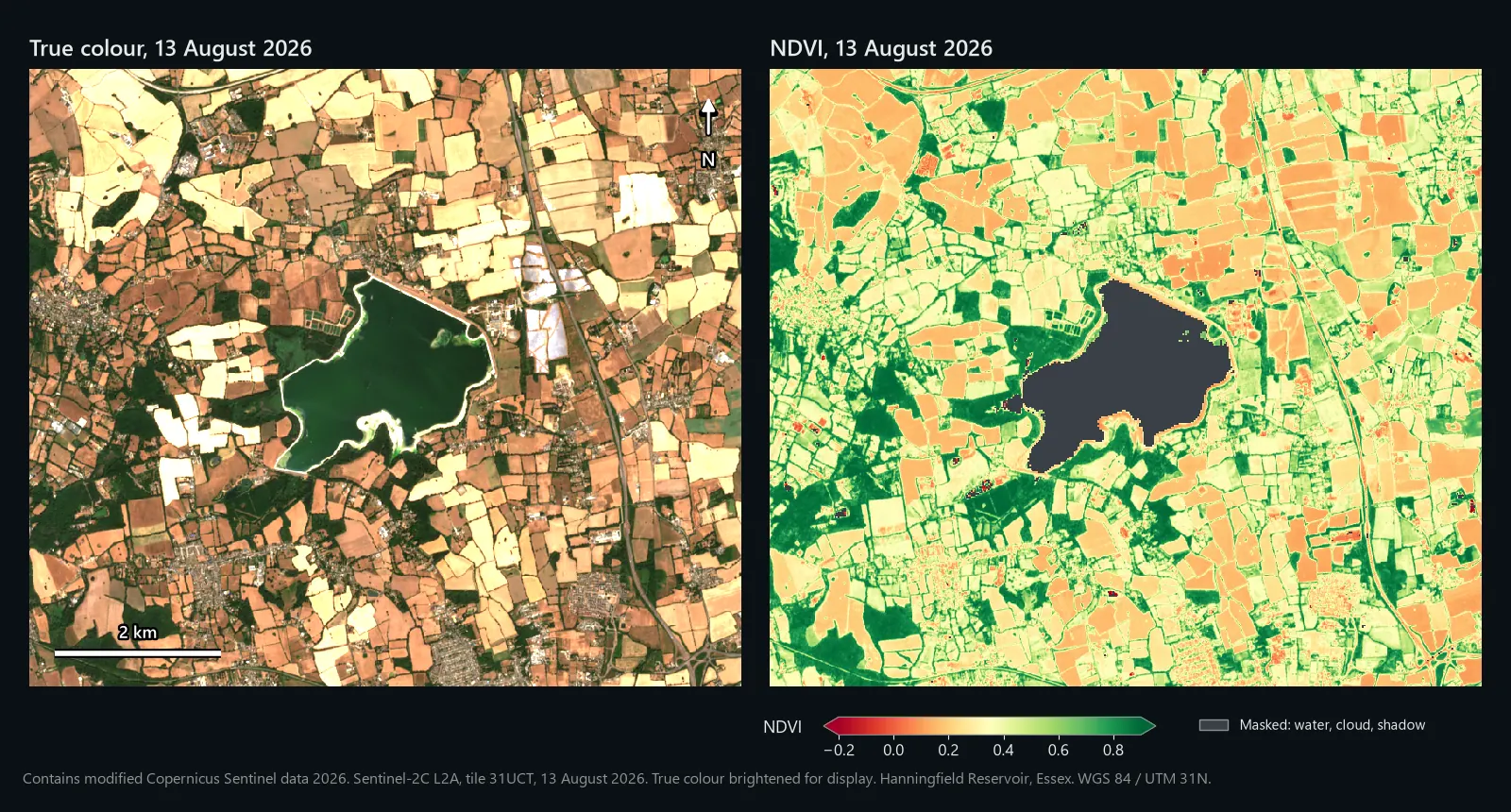
The worked example is the farmland around Hanningfield Reservoir, south of Chelmsford in Essex, on 24 June and 13 August 2026. We ran every step below in QGIS 3.44, with the same algorithms the menus call, on the two Copernicus products a reader would download, and every number here comes from those runs. The figures are drawn from the QGIS outputs.
What NDVI measures
Green leaves absorb most red light and reflect a lot of near-infrared (NIR). Soil, water and buildings do not show that contrast. The Normalised Difference Vegetation Index turns it into one number per pixel:
The result falls between -1 and +1. Dense green vegetation sits high, bare ground low, and water is usually negative. On Sentinel-2, red is band 4 (B04) and NIR is band 8 (B08), both at 10 m.
What you need
- QGIS 3.44. Any recent 3.x release works; menu names here are from 3.44.
- A free Copernicus Data Space Ecosystem account to download from Copernicus Browser.
- Your area of interest as a polygon layer, ideally field boundaries in a GeoPackage.
- Disk space for a large zip per date: each product covers a whole 110 km tile.
Step 1: choose the right product
Level-1C is top-of-atmosphere reflectance: what the satellite saw, haze included. Level-2A is atmospherically corrected surface reflectance, and it ships with a Scene Classification Layer (SCL) that flags cloud, shadow and water. Use L2A.
| Band | What it is | Resolution | Where it is in the product |
|---|---|---|---|
| B04 | Red | 10 m | IMG_DATA/R10m/..._B04_10m.jp2 |
| B08 | Near-infrared | 10 m | IMG_DATA/R10m/..._B08_10m.jp2 |
| SCL | Scene classification | 20 m | IMG_DATA/R20m/..._SCL_20m.jp2 |
B04 also appears in the R20m and R60m folders as a resampled copy, so take it from R10m. B8A is a narrower NIR band at 20 m; stay with B08 for 10 m pixels.
Step 2: download a scene from Copernicus Browser
- Open browser.dataspace.copernicus.eu and sign in.
- In the Visualize tab, choose Sentinel-2 L2A, lower the maximum cloud cover and step through the calendar until your area is clear. Judge the cloud over your fields, not the tile figure.
- In the Search tab, tick Sentinel-2 > MSI > L2A, set the time range to that day and press Search.
- Click the download icon on the product. You get a zip containing a
.SAFEfolder.
The product name carries what matters. Ours was S2C_MSIL2A_20260624T110621_N0512_R137_T31UCT_20260624T144908: Sentinel-2C, Level-2A, 24 June 2026, processing baseline 05.12 (N0512), relative orbit 137 (R137), tile 31UCT.
Step 3: load and clip the bands
- Unzip the product and open
GRANULE/L2A_T31UCT_.../IMG_DATA. Drag B04 and B08 fromR10mand SCL fromR20minto QGIS. - Check the CRS in Layer Properties > Information. Tiles use WGS 84 / UTM: 31UCT is EPSG:32631, and much of Great Britain falls in zone 30 (EPSG:32630).
- Run Raster > Extraction > Clip Raster by Mask Layer on each band with your polygon as the Mask layer. Tick Keep resolution of input raster and enter
0in Assign a specified NoData value to output bands. Then open Advanced Parameters and type-srcnodata 0in Additional command-line parameters. Save asB04_jun.tif,B08_jun.tifandSCL_jun.tif. Run as Batch Process does all three at once.
Zero means "no data" in L2A files, along swath edges for example, but the .jp2 files do not declare it. The NoData box on its own only marks the area outside your polygon: GDAL changes any zeros inside it to 1, and they come through as real values. -srcnodata 0 tells GDAL that the zeros in the source are no data. We tested both on a 2 km square across the swath edge of our tile: without it, 19,354 edge pixels came out as 1; with it, all 19,354 were NoData.
Step 4: check whether the offset is in your values
Since processing baseline 04.00 came in on 25 January 2022, ESA adds 1,000 to every stored L2A value, so that slightly negative reflectances over very dark surfaces are kept instead of clipped. To get surface reflectance:
The 10,000 cancels out in NDVI because it is a ratio. The 1,000 does not: NIR minus Red is unchanged, but NIR plus Red is 2,000 too big, which drags every value towards zero.
Go by the baseline in the product name, not the image date. N0400 or higher means the offset is in the files, and reprocessed older scenes can carry a newer baseline. The metadata file MTD_MSIL2A.xml, at the top of the .SAFE folder, states it: ours lists BOA_ADD_OFFSET as -1000 for every band (the amount you add) and BOA_QUANTIFICATION_VALUE as 10000.
Some cloud mirrors and download services remove the offset before you see the data, so check the numbers. Click open water in the B08 layer with Identify Features:
- Around 1,000 (a little either side over very dark water): the offset is in. Use the first formula in step 5.
- Near zero, up to a couple of hundred: already removed. Use the plain formula.
- Decimals between 0 and 1: already reflectance. Use the plain formula.
We checked two copies of the same 24 June scene. In the Copernicus file, B08 over the reservoir had a median of 1,008. In the copy on the Earth Search catalogue on AWS it was 8: the offset had already been removed, and negative values raised to 1. That catalogue's band metadata still lists a -0.1 offset, with only a separate flag saying it has been applied, so applying it again would be an easy mistake.
Step 5: calculate NDVI in the Raster Calculator
Open Raster > Raster Calculator and double-click layers in the Raster Bands list to add them. With the offset in:
That is the corrected formula with the 1,000s cancelled. If the offset was already gone:
Untick Create on-the-fly raster instead of writing layer to disk, save as ndvi_jun.tif, keep the extent and resolution matching B04, and click OK. The output is 32-bit float, so the decimals survive.
Step 6: mask clouds, shadows and water with the SCL band
The SCL gives every 20 m pixel a class. This is how we treated them:
| SCL value | Class | Use |
|---|---|---|
| 4, 5 | Vegetation, not vegetated | Keep |
| 6 | Water | Drop for a land study (see below) |
| 7 | Unclassified | Judgement call (we dropped it) |
| 2, 3 | Cast shadows, cloud shadows | Drop |
| 8, 9, 10 | Cloud medium probability, cloud high probability, thin cirrus | Drop |
| 0, 1, 11 | No data, saturated or defective, snow or ice | Drop |
Each comparison returns 1 or 0, so the bracket is 1 for clear land pixels and 0 for the rest. QGIS returns NoData when dividing by zero, so cloud, shadow, unclassified and water pixels drop out and the rest keep their value. The calculator resamples the 20 m SCL with nearest neighbour, which is right for classes; we checked our output pixel by pixel against the SCL. Take the extent, columns and rows from ndvi_jun so the output stays at 10 m, and save it as ndvi_jun_masked.tif.
Water goes because NDVI was designed for land, and dark water breaks it once the offset is removed. On 24 June the reservoir's near-infrared reflectance had a median of 0.0008, 46% of its pixels were below zero, and 46% of its NDVI values fell outside -1 to +1, some as far out as 139. Keep class 6 only if the water itself is your subject.
The mask can miss thin haze and cloud edges, so look at a true colour view too. Both our dates were almost cloud-free: cloud, shadow and unclassified pixels were 0.25% of the window in June and 0.15% in August, mostly unclassified, plus a little shadow and, in August, a few cloud and cirrus pixels. Water took another 5.1% and 4.7%.
Step 7: style it and read the values
- In Layer Properties > Symbology, set Render type to Singleband pseudocolor.
- Choose the RdYlGn colour ramp (it ships with QGIS), set Min to
-0.2and Max to0.9, Mode to Continuous, and Apply.
Use fixed values. The default cumulative count cut (2% to 98%) stretches each image to its own range, so two dates styled that way cannot be compared by eye.
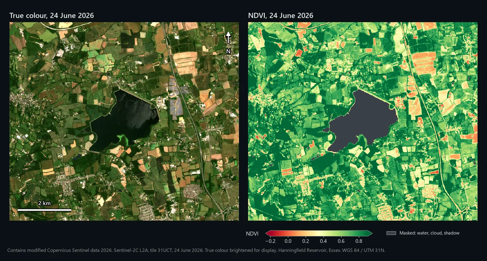
Treat NDVI ranges as rough guides: values shift with crop, growth stage, soil colour and sensor. The middle column follows NASA Earth Observatory's NDVI guide; the right column is what we measured.
| NDVI | Typical surface (NASA) | Our 24 June scene |
|---|---|---|
| 0.1 and below | Barren rock, sand or snow | 1.1% of the clear land pixels (water masked) |
| 0.2 to 0.3 | Shrub and grassland | Ground the SCL classed as not vegetated: median 0.24 |
| 0.6 to 0.8 | Temperate and tropical rainforest | Ground the SCL classed as vegetation: median 0.76 |
Step 8: get an NDVI value for each field
A map shows patterns; a report needs a number per field. In the Processing Toolbox, run Raster analysis > Zonal statistics with your field polygons as the Input layer, ndvi_jun_masked as the Raster layer, an Output column prefix such as jun_, and Count, Mean, Median and St dev ticked. NoData pixels are ignored, so a half-clouded field gets statistics from its clear half, and Count tells you how many pixels that was. Your polygons can stay in British National Grid: we ran it on 100 OpenStreetMap farmland polygons from the area, and QGIS matched them to the UTM raster itself. The 96 that overlap the raster got statistics; the four outside it got empty (NULL) values, not zeros.
If you do this for many parcels every season, our £1 NDVI Analysis model runs the NDVI, a low and high split and the per-parcel statistics in one go (details at the end).
Comparing two dates: NDVI change detection
Change detection here means subtracting one NDVI map from another. The care goes into making the two inputs comparable.
Step 9: pick a matching second scene
- Same tile, so both dates share a CRS and an identical pixel grid.
- Same relative orbit if possible, so the viewing angle matches.
- Same processing: offset handling and SCL classes kept.
Our second date, 13 August 2026, matched on satellite, tile (T31UCT) and orbit (R137). Run steps 3 to 6 again to get ndvi_aug_masked.
Step 10: subtract
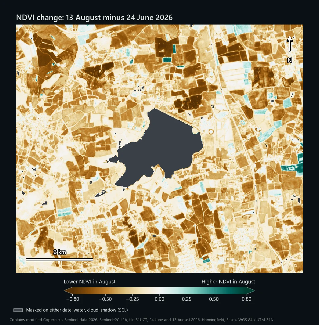
Later minus earlier, so negative values are losses, and a pixel masked on either date comes out as NoData. Save it as ndvi_change.tif and style it with the BrBG ramp from -0.8 to 0.8: brown is a drop, green a rise.
Step 11: put a number on it
That gives 1 for significant loss and 0 elsewhere. Run Raster analysis > Raster layer unique values report on it for the pixel count and area of each value (square metres on a UTM layer; divide by 10,000 for hectares). Over our 63.5 km² window, the report gave 88,139 pixels and 8,813,900 m² for value 1: 881 ha that dropped by 0.5 or more, 14.7% of the 6,003 ha of clear land.
99% of those pixels were classed as vegetation in June and as not vegetated in August. That is harvest: the true colour shows stubble and cultivated soil where green crops stood seven weeks earlier. The map shows where NDVI moved and by how much; the reason comes from context such as the crop calendar, the imagery or a site visit. A -0.5 threshold suits clear-cut events like harvest or clearance. Subtler stress needs a smaller one, tested where you know what happened.
The reservoir is the other lesson. With water left in the mask, the loss figure grew by 71 ha, almost all of it pixels the SCL called water in June, where the values were the out-of-range noise described in step 6. The water did change, though. By 13 August the true colour shows it had turned green, and its near-infrared reflectance had risen from a median of 0.0008 to 0.016. Read any NDVI change on water as a change in the water, not in vegetation.
Common problems
Wrong bands
B04 is red and B08 is NIR. Swap them and the sign flips: fields come out negative, water positive. If crops look red on RdYlGn, check the band order, then check both came from R10m.
Forgetting the offset
Nothing errors; NDVI just gets squashed towards zero. To show how much, we also ran the plain formula on the raw June bands:
| 24 June 2026 | Offset handled | Offset forgotten |
|---|---|---|
| Vegetation (SCL class 4, median) | 0.76 | 0.49 |
| Not vegetated (SCL class 5, median) | 0.24 | 0.15 |
| All clear land (mean) | 0.68 | 0.44 |
A healthy crop at 0.49 looks like it is struggling. Subtracting an offset that has already gone does the reverse and sends dark pixels wildly out of range. The step 4 check catches both.
Clouds, shadow and haze
A scene listed as nearly cloud-free can still have cloud over your patch, and cloud shadow ruins NDVI too. Use the SCL mask, look at the true colour, and if a field's Count from step 8 is low, find another date.
CRS mismatch between dates
Tiles overlap, and parts of eastern England are covered from both UTM zone 30 and zone 31. On 24 June 2026 our window came as T31UCT (EPSG:32631) and T30UYC (EPSG:32630); take one date from each and the rasters will not line up. Use the same tile for both dates. Failing that, run Raster > Projections > Warp (Reproject) with Target CRS set to match the other date and Output file resolution in target georeferenced units set to 10, then snap the grids together with Align rasters in the Processing Toolbox. Use Nearest Neighbour for the SCL.
NoData
If QGIS treats the zeros in L2A files as real values, they spread. With the offset formula, a pixel that is 0 in both bands gives 0 / -2000: a believable NDVI of exactly 0. Clipping without -srcnodata 0 turns those zeros into 1s, which gives the same believable 0. The step 3 setting prevents it, and the SCL mask catches anything left, because class 0 is no data. Layer Properties > Information shows a layer's NoData value, and the Transparency tab can add one for display.
Relatedly, very dark surfaces can have slightly negative reflectance once the offset is removed, and NDVI then leaves the -1 to +1 range. On our reservoir that was nearly half the pixels, which is why step 6 drops water. Values outside -1 to +1 across fields mean an offset mistake.
Credit the data
Copernicus Sentinel data is free, full and open, and the legal notice asks you to name the source. For processed outputs such as an NDVI map, use "Contains modified Copernicus Sentinel data [Year]". Unmodified data is "Copernicus Sentinel data [Year]".